
There are a number of programs widely available to prepare economic evaluations for
proposed investments. These programs typically use either simple payback and/or
discounted cash flow analysis. Unfortunately, these programs have often been
developed by governmental agencies or universities, which are not subject to income
taxes. As a result, they may ignore the impact of income taxes, which can influence
the outcome of economic analyses significantly. The discussion below illustrates the
effect of including income tax consequences in various forms of economic analysis.
Simple Payback
Using simple payback, the capital cost of a project is divided by the first year’s
expected savings to give an indication of how many years the project would take to
“pay back.” Economic analysts have railed against the use of simple payback for a
variety of reasons: it ignores the time value of money, it gives no credit for benefits
occurring after the payback period, etc. However, an equally damning aspect is
seldom mentioned: the fact that simple payback omits the effect of income taxes.
As a simple example, assume a proposed investment having the following
characteristics:
Tax Adjusted
Tax Life Payback Period
Five-year 5.1
15-year 6.4
39-year 7.2
Tax Life Payback Period
Five-year 5.1
15-year 6.4
39-year 7.2
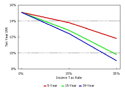
| Graph 1: Impact of Depreciation Schedule and Tax Rate on IRR |
Graph 1 shows how the expected return on an investment declines at higher tax rates
and longer depreciation schedules. If the proposal in question were for new HVAC
equipment to be purchased by an investor in a 35 percent marginal tax bracket, the
actual projected return on investment would be about nine percent. This is
substantially less than the 15-percent return projected when income taxes are
ignored.
The full impact of income taxes is probably best illustrated using net present value.
Using the same assumptions as above, and further assuming a ten-year study and a ten
percent discount rate, the results illustrated in Graph 2 were obtained.

| Graph 2: Impact of Depreciation Schedule and Tax Rate on NPV |
In this example, a project that appears to have positive economics when ignoring
income taxes may actually have a negative NPV when income taxes are properly
accounted for. In other words, by ignoring income tax consequences, an investor
could actually make an inappropriate investment decision.
In preparing NPV analysis, a few cautionary words about discount rate are in order.
First, it is important that if after tax cash flows are to be discounted, an after tax
discount rate must be used. Otherwise, an invalid NPV will result.
Secondly, the cost of borrowing money is probably not the appropriate discount rate,
even though this has been used in countless analyses. Because a company’s ability to
raise capital funds is limited, companies invest in a portfolio of projects based on the
expected returns and relatives risks of these projects. Projects must compete with
each other to be included in the portfolio of acceptable investments. Therefore,
when evaluating a proposal, the appropriate discount rate is the return that the
company would expect on a competing investment having similar risk. Tax treatment
for competing proposals may influence both their expected returns and perceived
risk.
[One final note: projects currently being planned and for which equipment has been
purchased after September 10, 2001, and which will be placed in service before
January, 2005, are allowed special tax treatment].
Investment $1,000,000
Electric savings $400,000
O&M Expenses $75,000
Fuel expenses $125,000
Net annual savings $200,000
Electric savings $400,000
O&M Expenses $75,000
Fuel expenses $125,000
Net annual savings $200,000
Calculating the simple payback as it is normally done:
| $1,000,000 ----------------- = 5.0 years $200,000 |
This calculation has two significant problems. First, it does not reduce the net
savings of $200,000 for the income taxes which must be paid. Secondly, it treats
the investment as though it were simply another expense, which could be written off
for tax purposes in the same year as the expenses for fuel and O&M.
In actuality, investments by tax-paying entities must be capitalized over a number of
years, adhering to schedules published by the IRS. The depreciation period varies
for different types of investments, referred to in the IRS Code as different kinds
of “property.” The depreciation period, or “tax life,” can vary from three to 39
years depending on: (1) what type of property is being depreciated, (2) how the
property is being used, and even (3) who owns the property.
To illustrate the complexity of selecting the correct tax life, consider that most
electric generating equipment is depreciated over a 15-year tax life, if it is not
owned by a public utility. However, if the electric generating equipment uses a
renewable fuel, such as hydro or biomass, the appropriate tax life is five years. A
condensing steam power plant owned by a public utility requires a 20 year tax life.
As another example, a chiller used in an industrial process can usually be depreciated
over a period dictated by the manufacturing process in which it is used -- usually
seven to ten years. On the other hand, a chiller used for space conditioning in an
office building would be depreciated over the same time frame as the building itself,
39 years.
The applicable tax rate may also not be obvious. It is important to use the investor’s
marginal tax rate for each new proposal. Any new project involves additional income
taxes, assuming it performs as expected and increases profits. Because these profits
are in addition to existing profits, the marginal, not average, tax rate should be used
for analysis.
Assuming a 35 income tax rate, (which would be close to what many companies pay,
including both Federal and state income taxes), the income tax adjusted payback
periods would increase from 5.0 years as follows:
It is clear from this table that income taxes can influence an investment’s projected
payback period significantly.
Discounted Cash Flow Analysis
Simple payback is typically used only as a quick screening tool to eliminate projects
which are clearly not worth pursuing further. Discounted cash flow analysis uses
more sophisticated indicators, such as internal rate of return (IRR) and net present
value (NPV). In determining these indicators of economic viability, tax consequences
are also critical.
Graph 1 illustrates the impact of different income tax rates and depreciation
schedules. Again using the assumptions noted above -- a $1,000,000 investment and
a $200,000 net annual savings -- we further assume that there is no inflation in
savings or expenses.
| Economic Evaluation -- A Taxing Exercise |